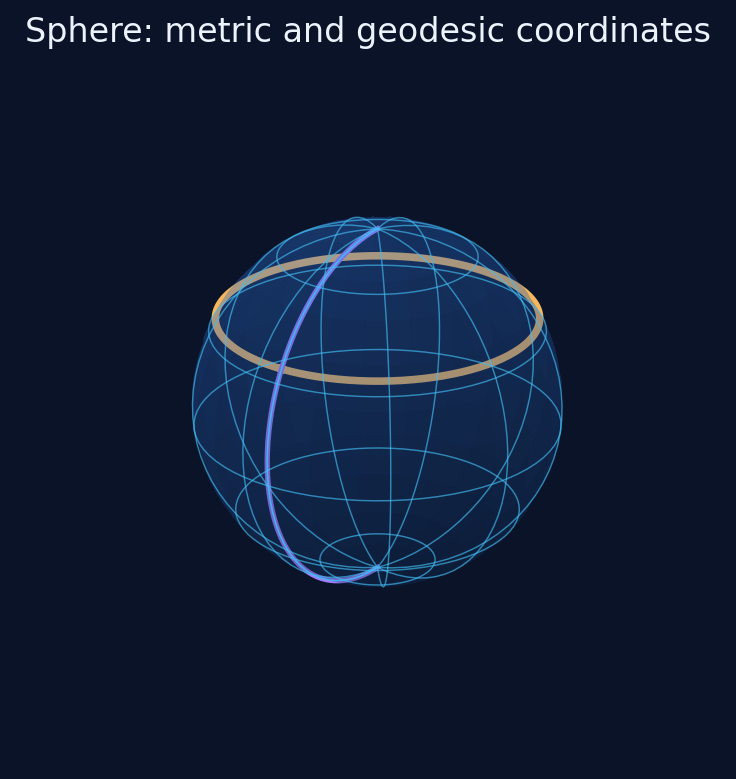
A metric on the sphere illustration
Numerical metric / standard sphere identity

A metric on the sphere

At a chosen latitude, the metric is an ordinary matrix. Its symbolic curvature remains a separate calculation.

theta=pi/3
g=[1,0;0,sin(theta)^2]
det(g)
inv(g)
Independently authored teaching example; Dean (1999), Chapters 2–4 provide geometric context.
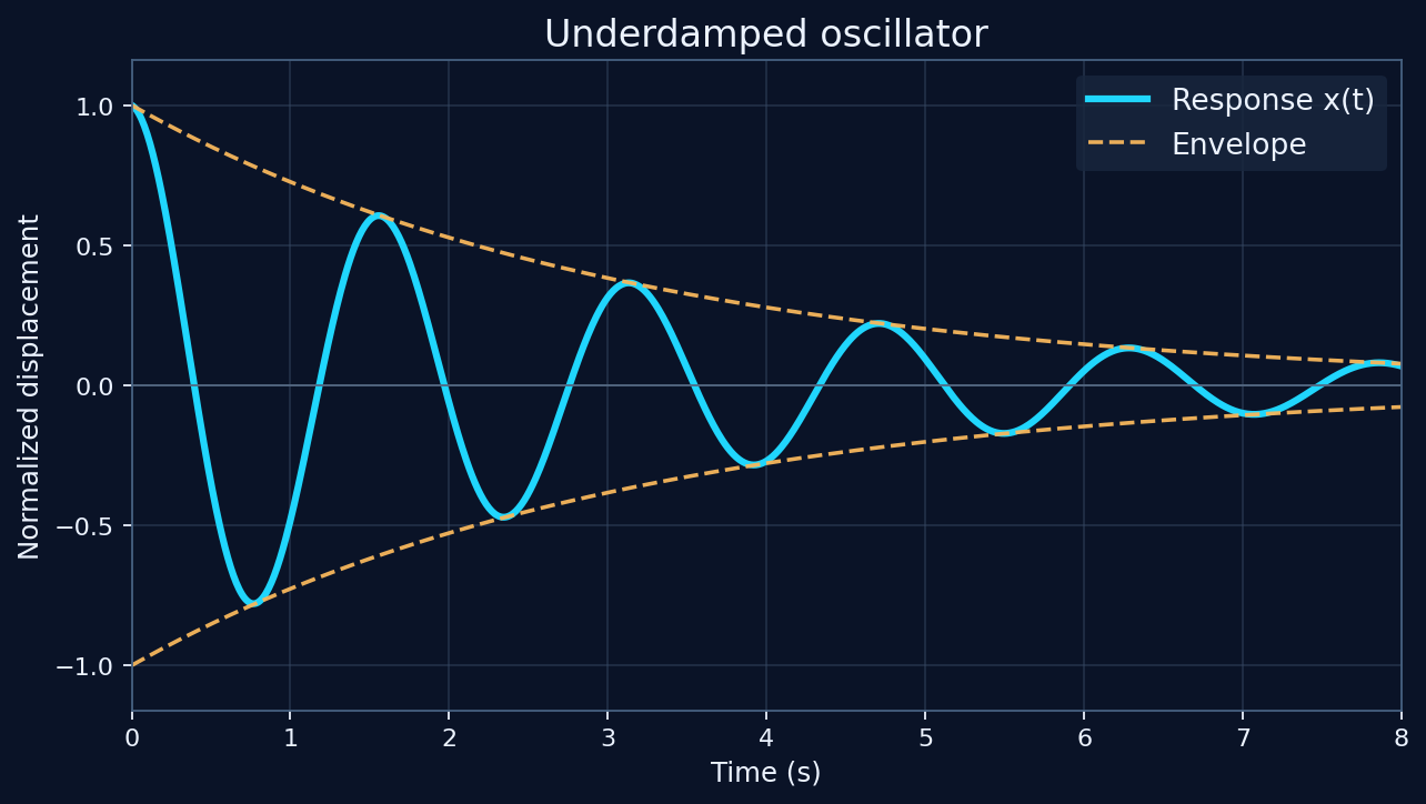
Damped mechanical response illustration
Vectorized numerical example

Damped mechanical response

Vectorized arrays let you compare a dynamic response against its envelope.

omega=4; zeta=0.08
t=linspace(0,8,401)
x=exp(-zeta*omega*t)*cos(omega*sqrt(1-zeta^2)*t)
plot(t,x,"Damped response")
Analytic linear-oscillator model; system identification is not implemented.
The symplectic matrix illustration
Source-based numerical check

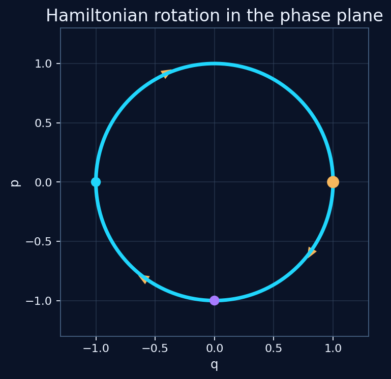
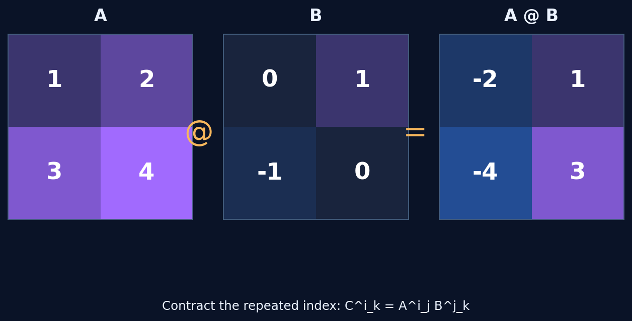
The symplectic matrix

The complex structure starts with a simple antisymmetric tensor from Hamiltonian mechanics.

J=[0,1;-1,0]
J@J
Dean (2026), Eq. (8) and Eqs. (11)–(13), pp. 4–5.
Binary Shannon entropy illustration
Vectorized numerical example

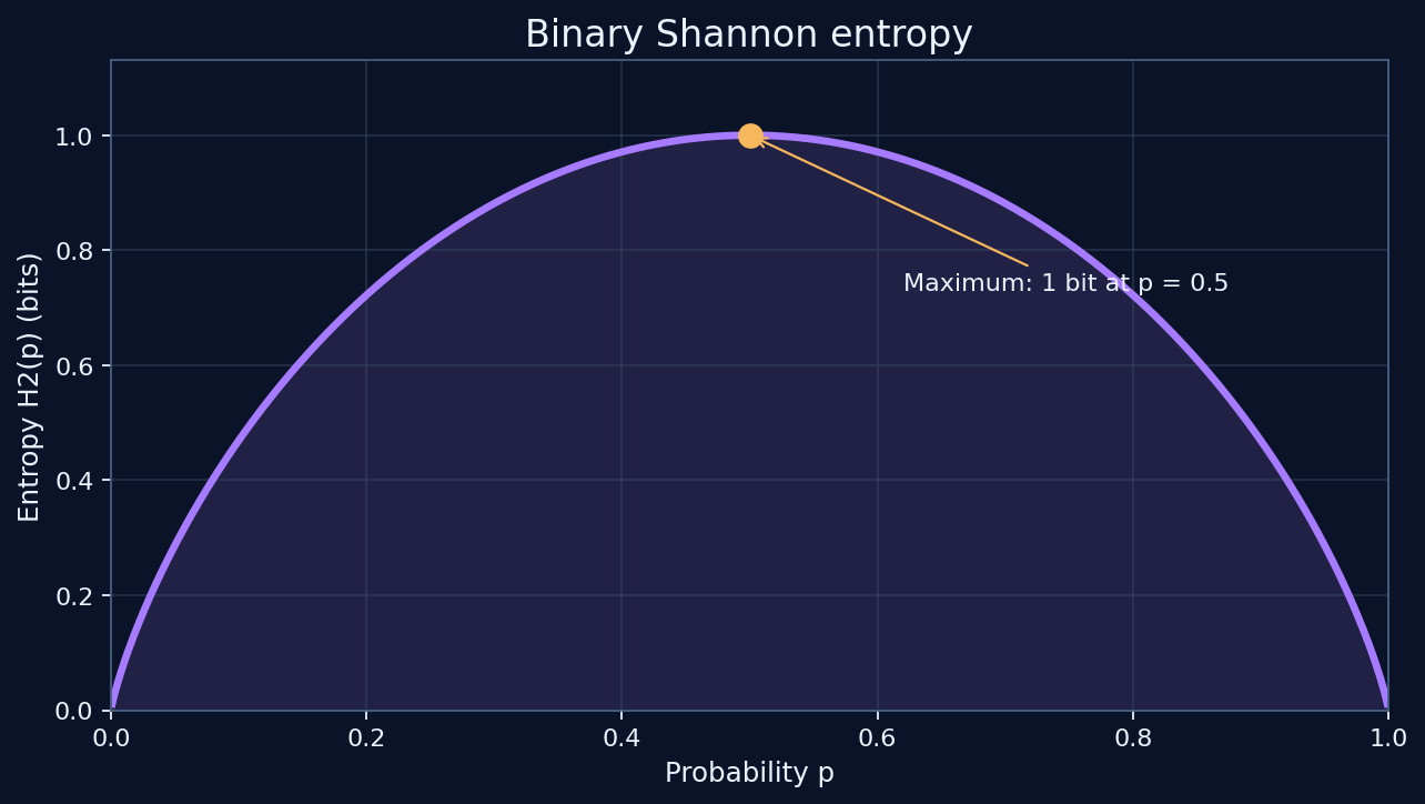
Binary Shannon entropy

A single expression generates an entire entropy curve.

p=linspace(0.01,0.99,199)
H=-(p*log2(p)+(1-p)*log2(1-p))
plot(p,H,"Binary entropy")
Shannon (1948), binary entropy; endpoint limits handled analytically.
Explicit metric and hybrid-index components illustration
Indexed numerical example

Explicit metric and hybrid-index components

Typed slots distinguish upper/lower variance from barred/unbarred conjugation.

h=metric([1,0;0,1],"V","hermitian")
u=indexed([1+i,2],"^a","V")
tinner(u,u,h)
# 6
Schouten convention discussed by Dean (2026), pp. 5–6; not full abstract tensor calculus.
Rotational gauge connection illustration
Source-based numerical check

Rotational gauge connection

A finite-dimensional numerical adaptation of the antisymmetric connection in a rotating frame.

W=[0,3,-2;-3,0,1;2,-1,0]
transpose(W)+W
W@[1,0,0]
Dean (1999), Appendix C, Eq. (C.9), pp. 166–168.
Correlated uncertainty illustration
Uncertainty-aware scalar check

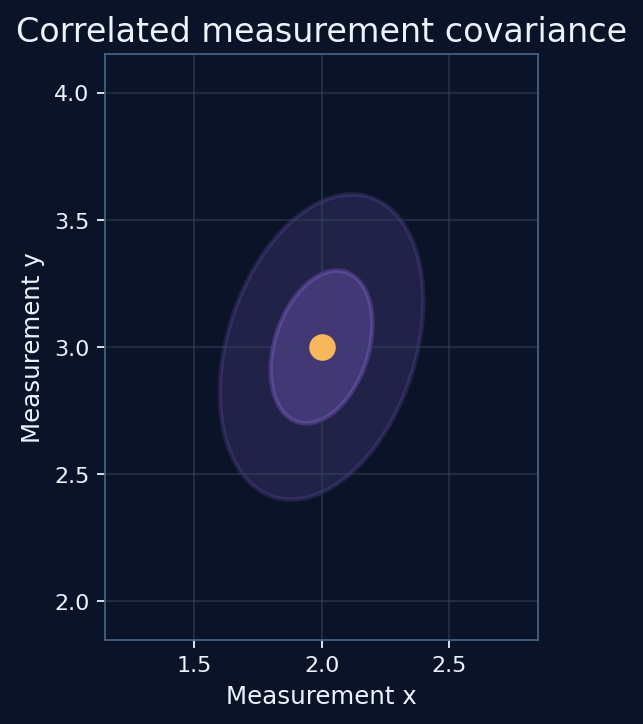
Correlated uncertainty

Measured inputs retain identity, so using the same variable twice preserves the dependency.

a=measure(2,0.1,"m")
sigma(a-a)
# 0
First-order propagation, not a guaranteed interval bound.