 Symbraix
The user guide
Mathematics, at hand.
Get started, find a function, or follow a worked example. One guide for light and dark, on any screen.
Symbraix 0.7 · November 2026
Search stays in this browser. No account required.
Contents
Learn with examples
- A small window for serious mathematics
- Your first calculation
- Scientific notation and variables
- Vectors, complex numbers and matrices
- Quantities that know what they mean
- A practical layer of algebra
- From expression to picture
- Tensor values and index metadata
- From Hamiltonian structure to complex variables
- Barred indices are geometric information
- Gauge kinematics from the dissertation
- A metric on the sphere
- A damped control response
- Dynamics in complex phase space
- Entropy in one line
- Know the limits of a result
- Settings, appearance and saved work
- Sources and reproducibility
Complete reference
- Keep it nearby
- Expressions and variables
- A scrolling calculation worksheet
- Complex arithmetic
- Vectors and broadcasting
- Matrices and elementwise calculations
- Linear algebra
- Function reference
- Additional scientific tools
- Precision and safe boundaries
- Sessions, privacy, and recovery
- Units and dimensional consistency
- Uncertainty and correlation
- Basic symbolic algebra
- Numerical tensor contractions
- Plot a calculation
- New, Open, and Save
- Recall complete commands
- Indexed tensors and metrics
- Hybrid indices and Hermitian metrics
- Change frames and preserve types
- Research references and development goals
01 / WHY WE BUILT IT
A small window for serious mathematics
We created Symbraix because a quick calculation should not require opening a programming environment, loading packages, or setting up an analysis notebook. We wanted mathematical depth without the overhead.
Symbraix stays alongside the work. A single expression can evaluate a trigonometric identity or a complex number; the same workspace can hold vectors, matrices, uncertainties, symbolic algebra, plots, and numerical tensor operations. We can revisit an earlier result without losing the context in which it was obtained.
Our ambition is broader than a calculator, but our interface remains deliberately modest. Symbraix is a focused scientific scratchpad for researchers, engineers, students, and anyone who thinks in equations.
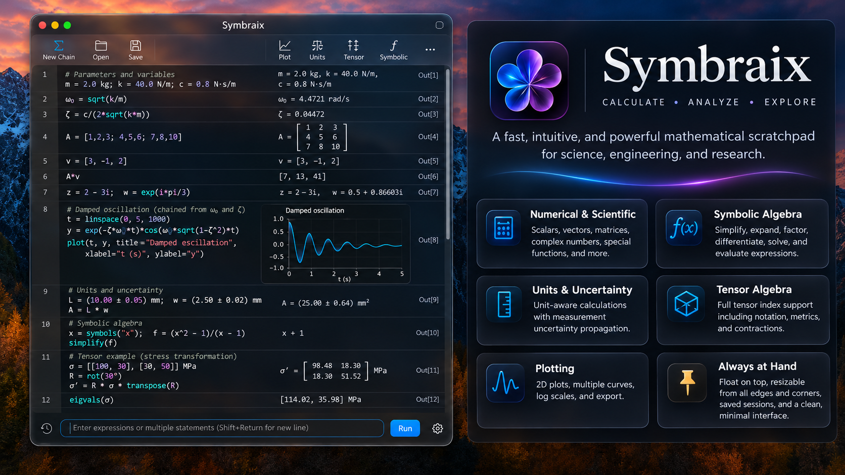
Concept artwork: a design illustration of the intended workflow, not a screenshot of the current TestFlight build.
02 / GET STARTED
Your first calculation
Open Symbraix. Type an expression in the lower editor, then press Return. Every successful statement becomes an item in the scrollable worksheet above.
vec(1,2,3,4) + vec(1,2,3,4)
Expected result or note: Result: [2, 4, 6, 8]
Definitions and evaluations can share one submission. Statements are separated by semicolons or new lines; semicolons inside square brackets remain matrix row separators.
x=4; y=7; x+y**2
Expected result or note: Results: 4, 7, 53
Shift-Return inserts a line without evaluating. Up/Down recall earlier commands at editor boundaries, while Option-Up/Option-Down explicitly cycle command history. Existing results are labelled Out[n]; out(n) reuses their full stored values.
| Control | Purpose |
|---|---|
| New / Command-N | Begin a fresh calculation worksheet |
| Open / Command-O | Open a previously saved chain file |
| Save / Command-S | Save the current chain, including results |
| Settings / Command-, | Set input and output text sizes independently |
| Keep on Top | Keep the calculator visible beside other apps |
The examples in this guide use a readable input syntax and are not a promise of arbitrary Python compatibility.
03 / EXPRESSIONS
Scientific notation and variables
Expressions are deterministic. Names store results, not live formulas; later reassignment does not rewrite old entries. Built-in functions use radians unless they explicitly specify degrees.
q=2; p=3
z=(q+i*p)/sqrt(2)
z*conj(z)
Expected result or note: Result: 6.5
| Notation | Interpretation |
|---|---|
| ^ and ** | Exponentiation; 2^3^2 evaluates as 512 |
| i or j | Imaginary unit, i*i = -1 |
| pi, e, tau | Mathematical constants |
| sin, cos, tan, exp | Elementwise numerical functions |
| ln, log2, log_10 | Logarithms by base |
| ans | Most recent successful result |
| out(n) | Saved full-precision worksheet result |
A malformed statement leaves its input available for correction. The worksheet and variable state of that submission are rolled back together, avoiding partially applied calculations.
04 / LINEAR ALGEBRA
Vectors, complex numbers and matrices
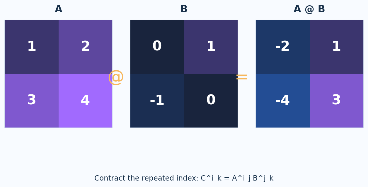
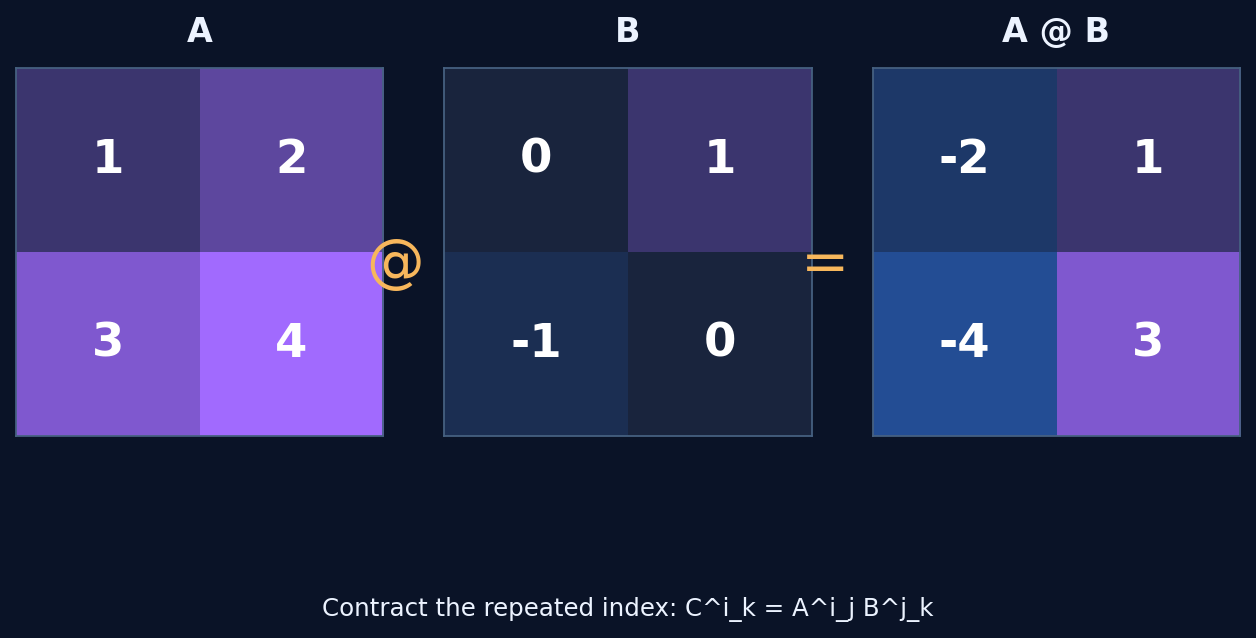
Array operations follow a NumPy-like distinction: * is elementwise multiplication and @ is matrix multiplication. The transpose is not the complex adjoint.
A=[1,2;3,4]
A*A
A@A
det(A)
inv(A)
Expected result or note: [[1,4],[9,16]] · [[7,10],[15,22]] · -2 · [[-2,1],[1.5,-0.5]]
Complex operations extend through vectors and matrices, including multiplication, conjugation and supported scientific functions. For inner products, dot(a,b) is bilinear, whereas vdot(a,b) conjugates its first argument.
u=[1+i,2]
vdot(u,u)
transpose(A)
adjoint(A)
Expected result or note: 6 · ordinary transpose · conjugate transpose
Some numerical factorization operations have size limits. The algebra engine is not a general matrix-function or arbitrary-precision package.
05 / UNITS & ERRORS
Quantities that know what they mean
Dimensional compatibility is checked when quantities are added or converted. Measurements carry standard uncertainties through supported operations using first-order derivative propagation.
length=measure(2,0.01,"m")
width=measure(30,0.2,"cm")
convert(length*width,"m^2")
Expected result or note: 0.6 +/- 0.005 m^2
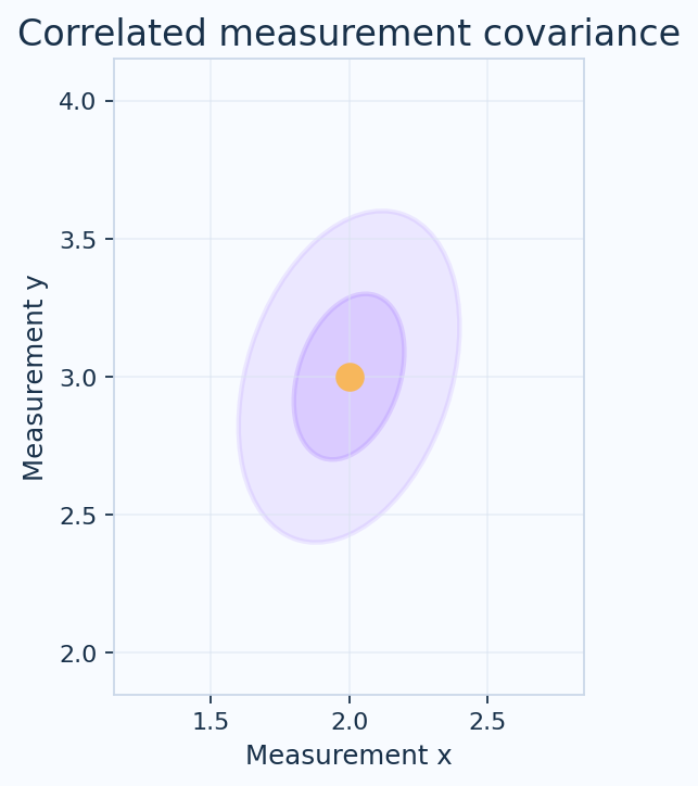
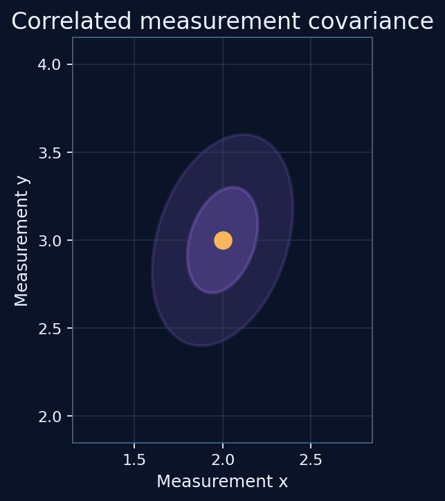
Reusing a measurement retains its identity and therefore its correlation. Two separately constructed measurements are independent unless an explicit correlation is provided.
a=measure(2,0.1,"m")
sigma(a-a)
sigma(a+a)
Expected result or note: 0 · 0.2
06 / SYMBOLIC
A practical layer of algebra
Symbolic expressions are constructed explicitly. This avoids confusing a misspelled numerical name with a new mathematical indeterminate. The supported manipulations are intentionally conservative.
simplify("2*x+3*x")
expand("(x+1)^2")
differentiate("x^3+2*x","x")
evaluate("x^2+1","x",[1,2,3])
Expected result or note: 5*x · expanded polynomial · 3*x^2+2 · [2,5,10]
The symbolic system handles a defined subset of simplification, expansion, substitution, differentiation and low-degree polynomial analysis. It does not automatically prove identities that depend on complex branches, positive-definiteness, or unspoken assumptions.
General-purpose symbolic tensor canonicalization, arbitrary symbolic integration and metric variation remain development goals rather than capabilities of the current beta.
07 / PLOTTING
From expression to picture
Define data in the same worksheet, then plot it directly. The plot captures the data as they were calculated; later changes to a variable do not alter the earlier result.
t=linspace(0,8,401)
omega=4; zeta=0.08
x=exp(-zeta*omega*t)*cos(omega*sqrt(1-zeta^2)*t)
plot(t,x,"Damped response")
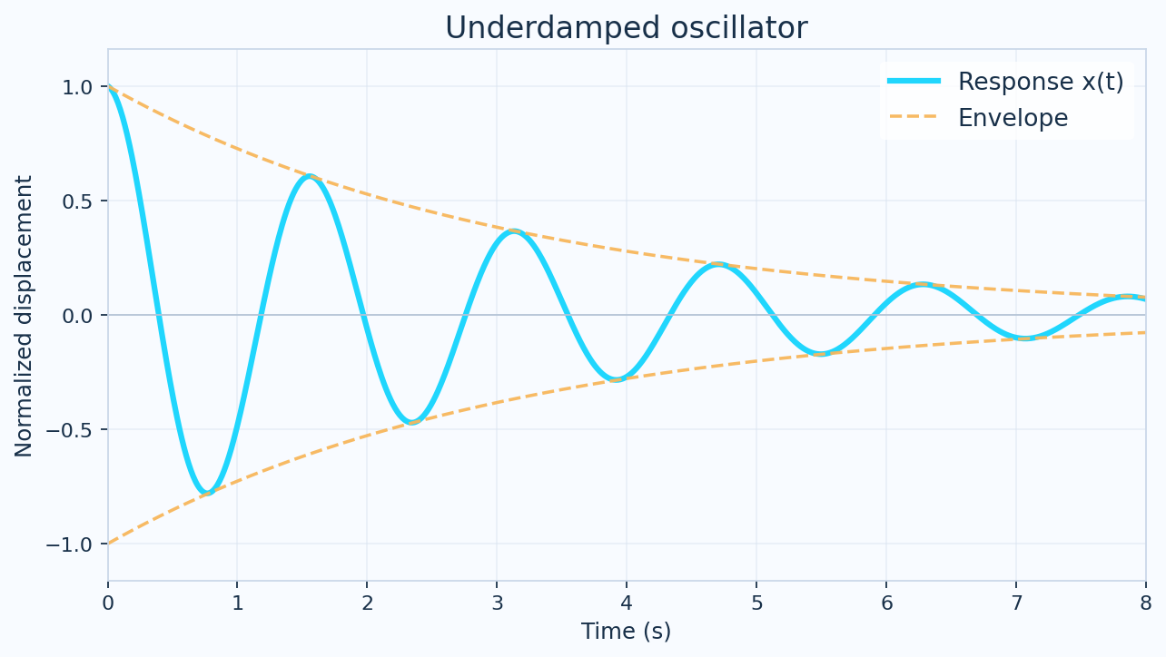
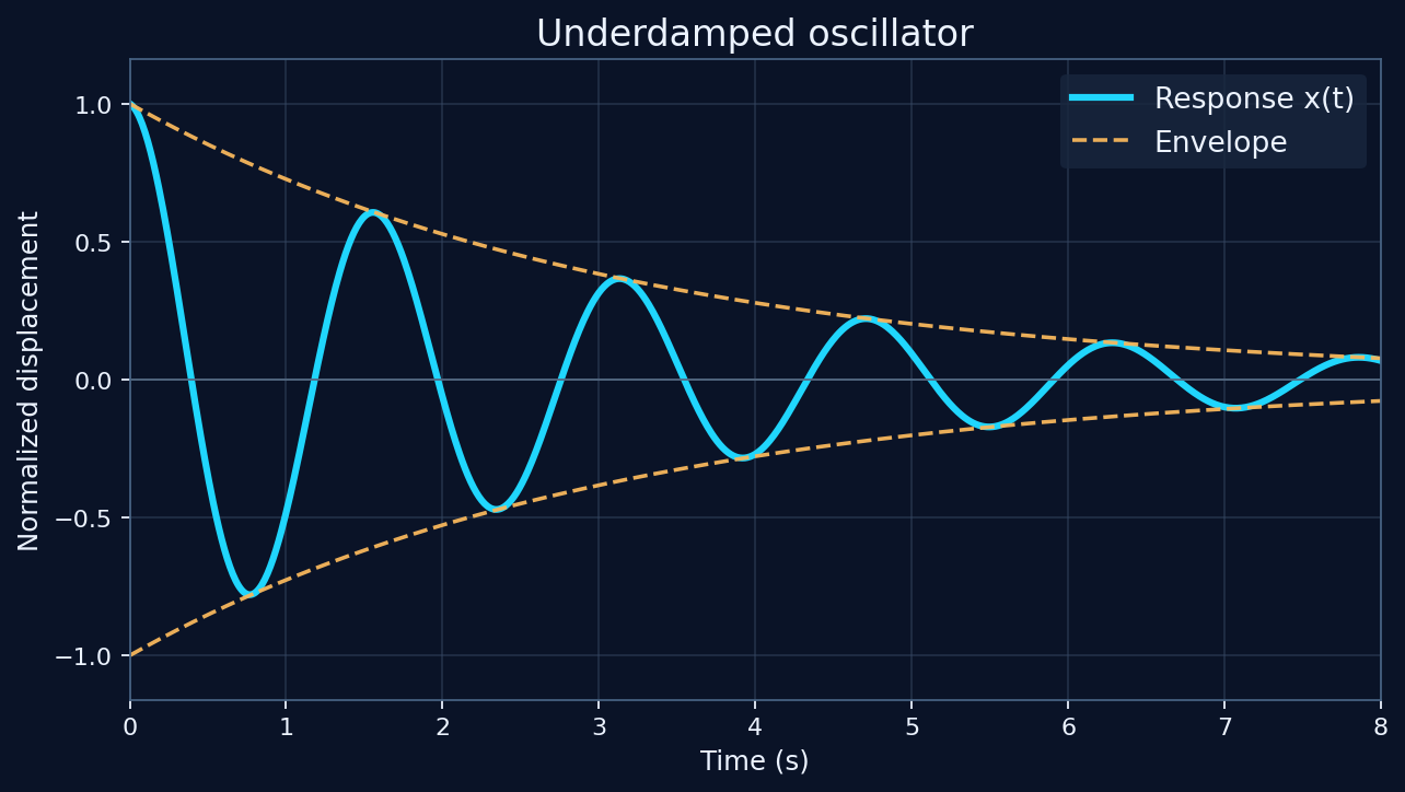
Line/scatter display, multiple curves and SVG figure export are supported in the underlying beta source. Plotting is sampled, not guaranteed to detect every discontinuity between samples.
08 / TENSORS
Tensor values and index metadata
Array rank alone is not enough for geometric tensor algebra. Our typed numerical tensor layer records index variance (upper/lower), conjugation kind (barred/unbarred), and a named carrier space.
| Text notation | Interpretation |
|---|---|
| ^a | Upper, unbarred index |
| _a | Lower, unbarred index |
| ^~a | Upper, barred index |
| _~a | Lower, barred index |
h=metric([1,0;0,1],"V","hermitian")
u=indexed([1+i,2],"^a","V")
tinner(u,u,h)
Expected result or note: 6
Other operations include component extraction, slot permutations, transposes, raising/lowering with explicit forms, compatible contraction, and numerical frame changes. Barred indices are not merely a synonym for covariant indices.
09 / SOURCE EXAMPLE
From Hamiltonian structure to complex variables
Dean (2026), Hamilton's equations in unitary form, Eq. (8), begins with the antisymmetric 2×2 tensor that organizes a coordinate-momentum pair. A direct numerical check is:
J=[0,1;-1,0]
J@J
J@[2,3]
Expected result or note: [[-1,0],[0,-1]] · [3,-2]
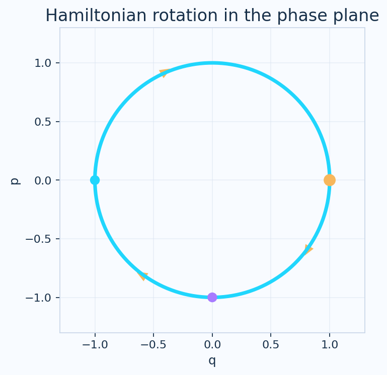
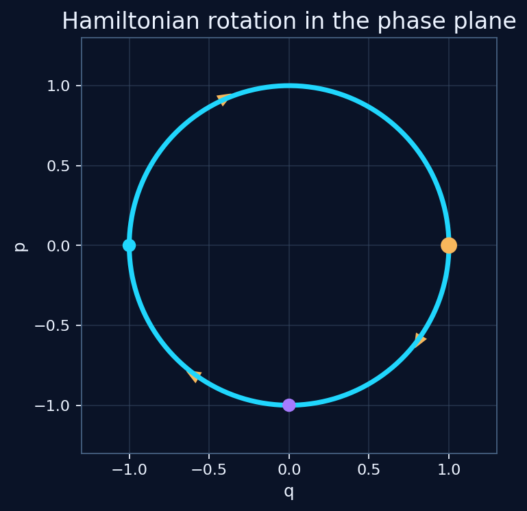
The matrix identity J² = −I explains the appearance of eigenvalues ±i. The manuscript's Eq. (13) defines complex variables from q and p; an executable scalar version is z=(q+i*p)/sqrt(2).
Source: Dean (2026), pp. 4–6, Eqs. (8), (11)–(16). Numerical checks supported; full symbolic derivation not claimed.
10 / SCHOUTEN NOTATION
Barred indices are geometric information
Dean (2026), p. 5, draws on J. A. Schouten's hybrid-index notation to place conjugation on the index rather than only the component symbol. This is distinct from upper-versus-lower variance. Symbraix therefore records these as separate slot attributes.
h=metric([1,0;0,1],"V","hermitian")
u=indexed([1+i,2],"^a","V")
tinner(u,u,h)
Expected result or note: 6
The example above illustrates a standard positive Hermitian form. It is not an assertion that the special transformed tensor in the manuscript's Eq. (14) is identical to the identity Hermitian form.
Sources: Dean (2026), pp. 5–6, Eqs. (13)–(16); Schouten (1954), as cited in that article.
11 / SOURCE EXAMPLE
Gauge kinematics from the dissertation
Dean's 1999 dissertation, Appendix C, develops a rotational gauge connection and its relation to motion in a rotating frame. The printed connection matrix in Eq. (C.9) is antisymmetric.
For a particular angular-velocity choice, the following is a straightforward component test following the sign convention displayed in that equation:
W=[0,3,-2;-3,0,1;2,-1,0]
transpose(W)+W
W@[1,0,0]
Expected result or note: Zero matrix · [0,-3,2]
This verifies antisymmetry and matrix-vector action, not the gauge-transformation law or a variational identity. Reproducing Eq. (C.10), the covariant derivative and full local SO(3) kinematics symbolically would require the extended tensor-field engine.
Source: Dean (1999), Appendix C, pp. 166–168, Eqs. (C.5)–(C.13). Numerical component adaptation.
12 / DIFFERENTIAL GEOMETRY
A metric on the sphere
On a unit sphere with coordinates (θ, φ), the standard two-dimensional metric is diag(1, sin²θ). Symbraix can evaluate its numerical components and inverse at a selected point.
theta=pi/3
g=[1,0;0,sin(theta)^2]
det(g)
inv(g)
Expected result or note: 0.75 · [[1,0],[0,1.333333...]]
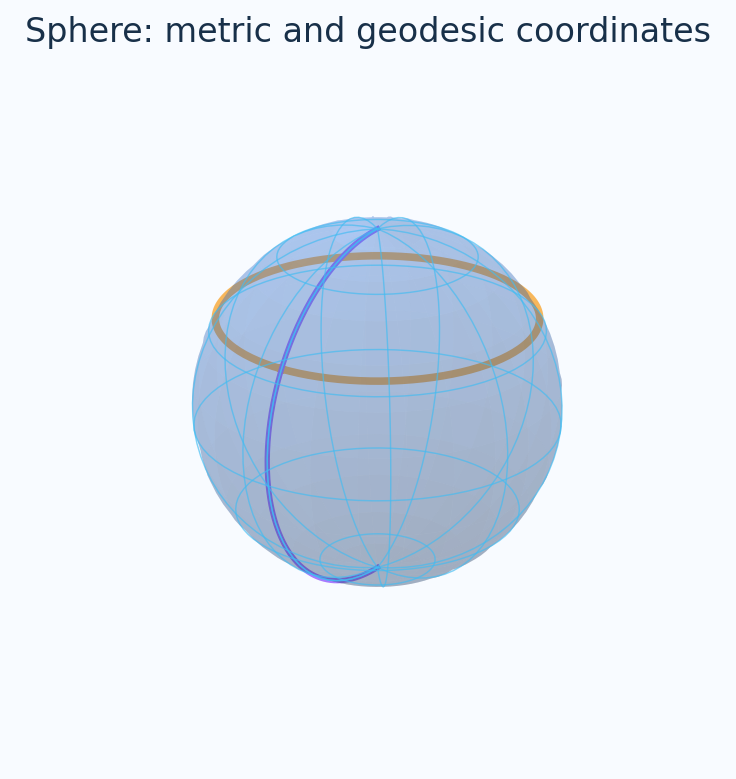
For a sphere of radius R, the Gaussian curvature K = 1/R² is a mathematical reference result. Automatically deriving the Christoffel symbols and curvature from an arbitrary symbolic metric is not a verified Build 8 feature.
Reference: Standard sphere metric. The related geometric motivation appears in Dean (1999), Chs. 2–4; this specific sphere example is an independently authored teaching example.
13 / ENGINEERING
A damped control response
A second-order underdamped system has a response with an exponentially decreasing envelope and a damped natural frequency. A vectorized workflow makes it easy to inspect its sensitivity to parameters.
omega=4; zeta=0.08
t=linspace(0,8,401)
wd=omega*sqrt(1-zeta^2)
x=exp(-zeta*omega*t)*cos(wd*t)
plot(t,x,"Damped response")
Unit-aware quantities and correlated measurements can be used separately for calibration. A complete symbolic transfer-function or robust-control toolbox is outside this initial beta.
14 / PHYSICS
Dynamics in complex phase space
The complex coordinate z = (q+ip)/√2 in Dean (2026), Eq. (13), joins a real phase-space pair for a chosen normalization. For a harmonic oscillator, the motion takes the form z(t)=z(0)e^(−iωt) in Eq. (28).
omega=2; t=linspace(0,2*pi,501)
z0=1+0.5*i
z=z0*exp(-i*omega*t)
plot(real(z),imag(z),"Complex trajectory")
This example exercises complex vectorization and 2D plotting. It does not, by itself, establish invariance under arbitrary canonical transformations or symbolic Poisson-bracket identities.
Source: Dean (2026), Section VI, pp. 8–9, Eqs. (25)–(29).
15 / INFORMATION THEORY
Entropy in one line
The binary Shannon entropy measures uncertainty in a Bernoulli variable with probability p, in bits:
The calculator can evaluate the expression elementwise. Avoid p=0 or 1 with direct logarithms and evaluate the limiting values separately.
p=linspace(0.01,0.99,199)
H=-(p*log2(p)+(1-p)*log2(1-p))
plot(p,H,"Binary entropy")
Expected result or note: At p=0.5, H = 1 bit
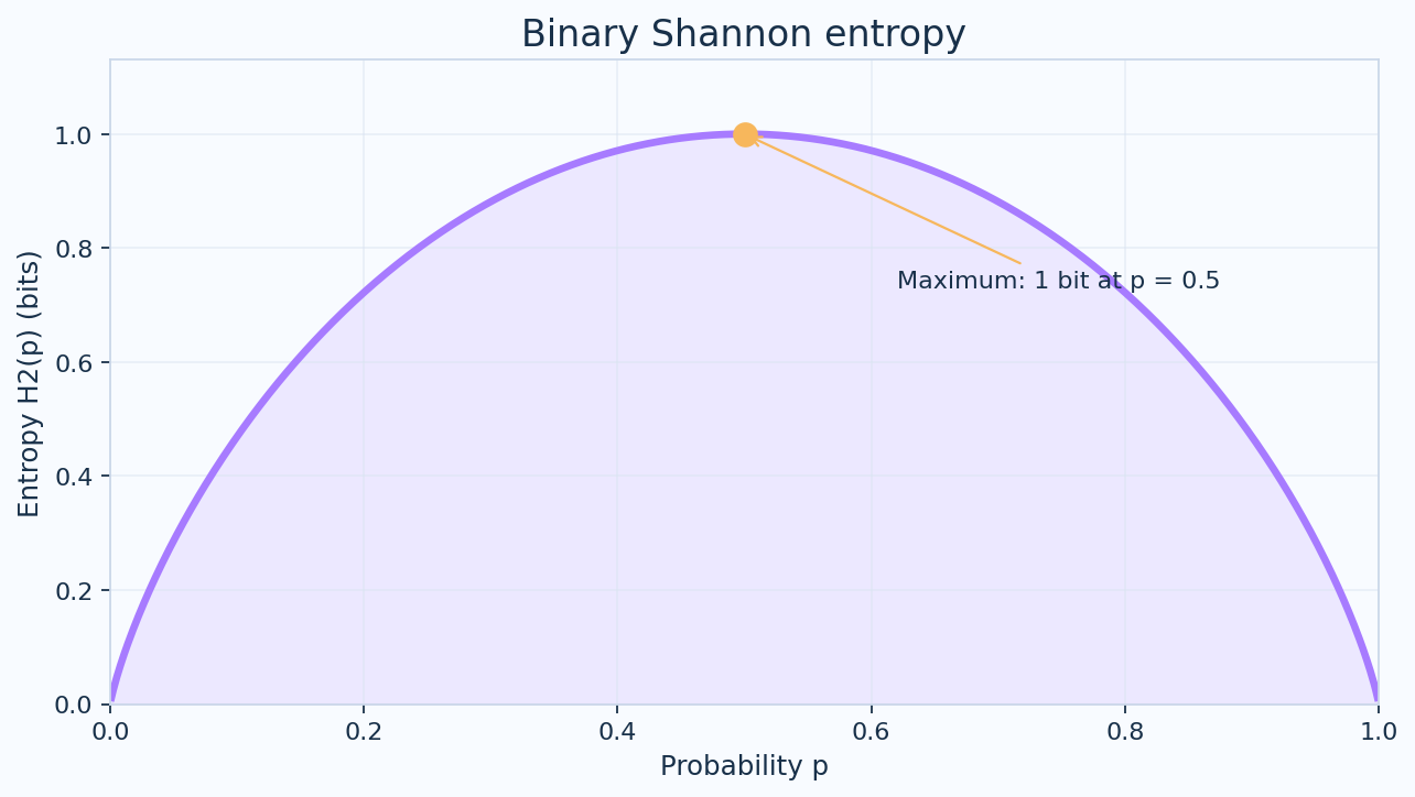
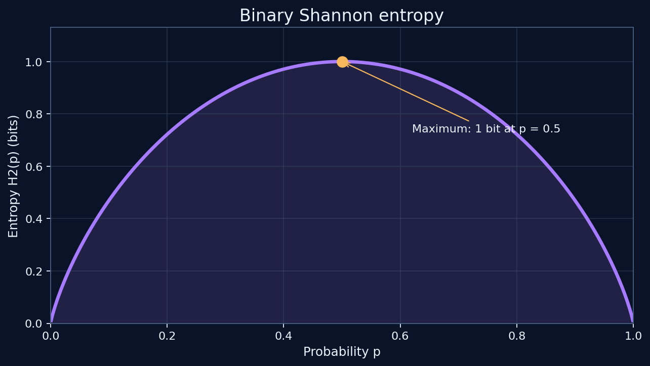
This is a useful example of mathematical depth without a specialized statistics or communications interface. More elaborate channel-coding and inference algorithms are outside the release scope.
Reference: Shannon (1948), A Mathematical Theory of Communication, Bell System Technical Journal.
16 / NUMERICAL INTEGRITY
Know the limits of a result
Symbraix uses standard floating-point computations for most numerical values. It aims for deterministic and explainable behavior, but it is not a certified arbitrary-precision or interval-arithmetic system.
| Area | Current boundary |
|---|---|
| Floating point | 64-bit real and complex values |
| Vector/matrix/tensor | Finite numerical arrays with shape and resource limits |
| Symbolic manipulation | Restricted algebra; no full CAS assumptions engine |
| Tensor algebra | Index-aware components; incomplete abstract tensor calculus |
| Uncertainty | First-order scalar error propagation |
| Plots | Sampled two-dimensional data; no adaptive guarantee |
Retain the source expression, units, coordinate conventions, and error assumptions for any result used in design, publication, or safety-related work. Numerical comparisons should use stated tolerances, not equality of displayed decimal strings.
Important research boundary: the supplied dissertation's MathTensor workflows for curvature variations, Palatini equations and complete Einstein-Hilbert symbolic derivations are not verified as supported in this beta.
17 / MANUAL & APP
Settings, appearance and saved work
Symbraix follows the system light/dark appearance. In the updated development source, Symbraix → Settings (Command-comma) contains independent font-size settings for input and worksheet results. These were still awaiting fresh interactive acceptance when the first macOS TestFlight Build 8 was uploaded.
New begins a calculation; Open restores a saved chain without reevaluating; Save writes the state of the worksheet and supported result values. Explicit file operations should not change appearance preferences.
This HTML Help system follows system appearance and includes the guide and detailed reference. In the updated app, choose Help → Symbraix Help to visit it, or Help → Quick Reference for a short offline reminder. The Light and Dark PDF manuals remain bundled in the updated application during this transition; existing installed builds change only when you update the app.
18 / SOURCES
Sources and reproducibility
Dean, Bruce H. (2026). Hamilton's equations in unitary form, manuscript dated September 17, 2026. Especially Secs. IV–VI and Eqs. (8), (11)–(16), (25)–(29). Supplied author manuscript.
Dean, Bruce Herold (1999). Variational Results and Solutions in Gauge Gravity and a Bifurcation Analysis of Black Hole Orbital Dynamics. Ph.D. dissertation, West Virginia University. Appendix A (MathTensor 2.2/Mathematica 3.0), Appendix C (gauge kinematics), Chapters 2–6.
Schouten, J. A. (1954). Ricci-Calculus, 2nd ed.; Tensor Analysis for Physicists, 2nd ed. Referenced in Dean (2026).
Christensen, S. M. and Parker, L. (1994). MathTensor: A System for Doing Tensor Analysis by Computer. Addison-Wesley. Referenced in Dean (1999).
Shannon, C. E. (1948). “A Mathematical Theory of Communication,” Bell System Technical Journal.
Symbraix 0.7.0 (8) documentation edition, November 2026. This guide accompanies a beta release; features may change before public distribution.
Complete reference
The detailed reference below preserves the original 0.7 manual. Historical edition labels are retained; the worked examples and mathematical limits remain part of this guide.
Complete reference
User Guide
Version 0.7.0 | Candidate 08 (build 8) | November 2026
We are developing Symbraix to make advanced mathematical analysis fast, intuitive, and easily accessible. Our goal is a minimal workspace that stays beside your work, from quick everyday calculations to symbolic expressions, units, uncertainty, and advanced tensor-index calculations, without the setup and visual complexity of a general programming environment.
Your first calculation
Open Symbraix, click the expression field when you are ready to type, and enter:
vec(1,2,3,4) + vec(1,2,3,4)Press Return. The result is:
[2, 4, 6, 8]No Python installation, package manager, account, or internet connection is needed for calculations. This is a native Mac app window, not a WidgetKit extension.
Find what you need
- Keep the calculator nearby and use the keyboard
- Expressions, variables, and the scrolling worksheet
- Complex numbers, vectors, and matrices
- Linear algebra and scientific function reference
- Precision, limits, privacy, and recovery
- Units and dimensional consistency
- Uncertainty and correlation
- Basic symbolic algebra
- Numerical tensor contractions
- Plots and figure export
- New, Open, and Save
- Command recall and indexed tensor algebra
Keep it nearby
Keep on Top is on by default for this version. The calculator stays above ordinary app windows when you switch to another application. It does not have to be selected in the Dock to remain visible. Typing still goes to the application you have chosen; floating does not capture your keyboard.
Move it once
Drag the empty part of the top header, beside the Symbraix name. Resize from any edge or corner, including the upper edge and upper corners. The expression and result remain selectable. We remember the window position and restore it when you reopen the app. If a display is disconnected, the calculator is moved back into an available screen area.
The filled pin indicates Keep on Top. Click it, or use Window > Keep on Top, to allow other windows in front. Your choice is remembered. The window requests availability across desktop Spaces; full-screen applications, Stage Manager, and system overlays remain subject to macOS window management.
Text size in Settings
Choose Symbraix > Settings… or press Command-comma, including while typing an expression. The small native Settings window opens above the pinned calculator. Opening Settings again brings the same window forward. Closing it leaves Keep on Top unchanged.
Input font size changes the active multiline editor. Calculation display font size changes existing and future worksheet expressions and text answers, including vectors, matrices, units, uncertainty, symbolic and indexed tensor results. The controls are independent, accept 10–36 points, and take effect immediately. Use the numeric field (Return to commit) or the stepper. Tab moves between controls.
The defaults preserve the earlier appearance: input 17 pt and calculation display 22 pt. The display value is the main answer size; expressions and matrix answers retain their smaller relative sizing, with a 10 pt minimum. Font families and alignment stay the same. Toolbar buttons and plot labels do not grow.
Changing fonts preserves your unfinished text, selection, text undo history and stored values. It does not calculate again. Long input wraps and scrolls; wide answers scroll horizontally and multiline answers grow vertically. Both preferences survive quitting and reopening. New, Open and Save affect calculations, not these app preferences. Restore Defaults resets only the two text sizes, without clearing calculations or changing pinning or window geometry.
Resize at the visible boundary
Drag the visible top, bottom, left or right border to change one dimension, or a rounded corner to change both. The opposite edge or corner stays anchored, subject to the minimum usable size and available screen area. A directional resize cursor distinguishes the boundary from the header interior. Drag the empty interior header beside the name to move the whole window. These gestures work with Keep on Top on or off; the resized geometry is remembered.
Close, hide, or quit deliberately
Changing apps does not close the calculator. Standard Mac controls still let you close, hide, or minimize it intentionally. Window > Show Symbraix, Command-0, the Dock icon, or the menu-bar entry restores it. Command-Q quits the app. There is no automatic login launch.
| Action | Keyboard |
|---|---|
| Evaluate all statements in the input | Return |
| Focus and select the expression | Command-L |
| Force older / newer command recall | Option-Up / Option-Down |
| Clear the current input, keep saved values | Escape |
| Copy the full last successful result | Command-Shift-C |
| Go to the latest calculation | Command-Y |
| Show the calculator while Symbraix is active | Command-0 |
| Close / minimize the current window | Command-W / Command-M |
| Settings | Command-comma |
| Quit Symbraix | Command-Q |
| Insert a new line without calculating | Shift-Return |
| Move within input; recall at its boundaries | Up / Down |
These are app shortcuts, not system-wide hotkeys. Use the menu-bar entry when another app is active. The interface follows system light or dark appearance; Reduce Transparency uses a solid background.
Expressions and variables
Enter assignments and expressions in order. Separate statements with semicolons or new lines. Return evaluates the current input; Shift-Return inserts a new line. The following can be entered separately or together:
| Input | Result |
|---|---|
x = 7 |
7 |
y = 4 |
4 |
x + y |
11 |
x + y = ? |
11 |
z = x + i*y |
7 + 4*i |
z^2 = ? |
33 + 56*i |
The optional suffix = ? (or simply ?) asks for evaluation. It is not an equation solver. An assignment such as x = 7 stores a value; an expression such as x + 4 = 7 does not solve for x.
Names store values, not live formulas
Names are case-sensitive. Use names such as x, velocity, or sample_2, beginning with a letter or underscore. Constants, function names, i, j, and ans are reserved. There can be up to 64 named variables. Reassigning an existing name replaces its value. Legacy saved variables that share a newly added function name remain usable; the variable name and a function call such as det(A) are distinct.
For example, after x = 7 and y = x + 1, y is 8. Changing x to 20 does not change y until you evaluate its assignment again. Recalling history reevaluates the expression using current variables, not the old values.
Operators and constants
| Syntax | Meaning |
|---|---|
| + - * / | Addition, subtraction, explicit multiplication, division |
| ^ or ** | Power, not bitwise XOR; 232 is 512 |
| -2^2 and (-2)^2 | -4 and 4, respectively |
| % | Real-number remainder with the divisor's sign |
| pi, e, tau, eps | Pi, Euler's number, 2*pi, binary64 epsilon |
| ans | The last successful result, including assignments |
Write 2pi or 3i, not 2pi or 3i. Use a decimal point and commas between arguments, independent of region settings. Scientific notation such as 1e-6 is supported. If any statement fails, no statement from that submission changes variables, ans, or the worksheet. Correct the highlighted input and evaluate again.
A scrolling calculation worksheet
The worksheet above the input keeps expressions and results in order. Scroll it to review earlier calculations. The input below it is a separate, scrollable multiline editor. It grows to seven lines and then scrolls; resize the window for more working space.
Define, calculate, continue
Type this on one line and press Return:
x = 4; y = 7; x+y**2The worksheet records three results: 4, 7, and 53. The input clears after success and keeps keyboard focus, ready for the next calculation. Alternatively, use Shift-Return between statements and Return once to evaluate the whole input.
Reuse an earlier answer
Each new result is labeled Out[n]. Click that label to insert out(n) at the input cursor, or type the reference yourself. It uses the stored value, not the rounded screen text. On a new session, the example above gives Out[3] = 53; out(3)*2 then returns 106. Use the actual number shown in your worksheet.
The reuse-arrow recalls an expression for evaluation with current variables. Out[n] instead inserts the saved value, including its uncertainty correlations. Copy Result produces reusable text for ordinary values. Copying a measurement creates an independent measurement when pasted; use Out[n] or Save when identity matters.
Separators and errors
Semicolons inside brackets remain matrix row separators: A=[1,2;3,4]; A@A is two statements. New lines inside brackets or parentheses are whitespace; keep a semicolon between matrix rows. Wrap a long expression in parentheses to continue it over several lines.
A failed submission keeps your input and reports the offending statement and location. None of its assignments or results is saved. Earlier successful work remains unchanged. Blank lines and trailing semicolons are accepted; a trailing semicolon does not suppress output. This is a sequential worksheet, not a reactive spreadsheet.
A submission supports up to 128 statements and shares one work budget. The worksheet retains up to 1,000 entries and 200,000 result elements, removing the oldest entries first. Result numbers are never reassigned while a session continues; an evicted out(n) reports an unavailable-result error. Assign important results to named variables.
Complex arithmetic
The constants i and j both represent the imaginary unit. They cannot be reassigned. Real and imaginary components each use 64-bit floating-point arithmetic.
| Input | Result |
|---|---|
i*i |
-1 |
z = 2 + 3*i |
2 + 3*i |
z^2 |
-5 + 12*i |
conj(z) |
2 - 3*i |
z*conj(z) |
13 |
real(z) / imag(z) |
0.666666666666667 |
sqrt(-1) |
i |
complex(2,3) |
2 + 3*i |
Components, magnitude, and phase
real(z) and imag(z) extract components. conj(z) (or conjugate(z)) takes the conjugate. abs(z) is the magnitude, and arg(z) (or phase(z)) is the phase in radians. phase(0) is defined as 0 in Symbraix. complex(a,b) constructs a + i*b from real inputs and broadcasts over vectors and matrices.
Branches are a deliberate convention
Complex square roots, logarithms, non-integer powers, and inverse functions return a principal value, not every possible value. For example, ln(-1) returns approximately pii and sqrt(-4) returns 2i. A negative real input can therefore produce a complex answer instead of a domain error.
Use an explicit small positive or negative imaginary component to approach either side of a branch cut. Exactly zero imaginary components are normalized to real values; signed-zero branch-side distinctions are not preserved in stored results. Tiny nonzero components are not silently discarded.
Integer powers use repeated multiplication, so i^2 is exactly -1. Expressions such as exp(i*pi) can retain a tiny imaginary rounding residual. cbrt(-8) returns the real cube root, -2; a genuinely complex input uses a principal cube-root value.
Complex numbers are not ordered. min, max, minimum, maximum, floor, ceil, round, sign, and % require real inputs. Select abs, real, or imag first when that is the operation you intend.
Vectors and broadcasting
Use vec(1,2,3), vector(1,2,3), array(1,2,3), or [1,2,3]. Elements can be real or complex. A vector is rank one. When it broadcasts against a matrix, it aligns with the matrix columns. Use reshape(v,n,1) to make an explicit column matrix.
| Input | Result |
|---|---|
[1,2,3] + [1,2,3] |
[2, 4, 6] |
[1,2,3]*2 + 1 |
[3, 5, 7] |
sqrt([1,4,9]) |
[1, 2, 3] |
[1+i,2-i] + i |
[1 + 2*i, 2] |
[1,2,3] * [4,5,6] |
[4, 10, 18] |
dot([1,2,3],[4,5,6]) |
32 |
norm([3*i,4]) |
5 |
linspace(0,1,5) |
[0, 0.25, 0.5, 0.75, 1] |
arange(1,5) |
[1, 2, 3, 4] |
Elementwise is the default
Arithmetic and ordinary scientific functions act on each element. A scalar or a length-one vector expands across the other vector. Otherwise lengths must match. Empty vectors are supported where the operation is defined. A shape error explains incompatible lengths.
Two different inner products
dot(a,b), or a @ b, sums a[k]b[k] without conjugation. vdot(a,b) sums conj(a[k])b[k]. Both require equal-length vectors and do not broadcast. This follows the NumPy distinction, not MATLAB's default complex dot convention.
a = [1+i, 2]
dot(a,a)     -> 4 + 2*i
vdot(a,a)    -> 6
Access and combine elements
Indexing starts at zero: [10,20,30][0] is 10 and [10,20,30][-1] is 30. concat joins vectors. diff returns successive differences; cumsum returns running sums. cross accepts two three-element vectors. Matrix rows and entries are described on the next page. Slices are not supported.
Matrices and elementwise calculations
Use [1,2;3,4] or [[1,2],[3,4]] for a two-row, two-column matrix. Inside brackets, semicolons separate rows and commas separate entries. Outside brackets, semicolons separate statements. All rows must have the same nonzero length. mat([1,2],[3,4]) is another spelling. Each entry may be real or complex.
| Input | Result |
|---|---|
A = [1,2;3,4] |
[[1, 2], [3, 4]] |
A + 10 |
[[11, 12], [13, 14]] |
A * A |
[[1, 4], [9, 16]] |
A @ A |
[[7, 10], [15, 22]] |
A^2 |
[[1, 4], [9, 16]] |
[i,2*i;3*i,4*i]^2 |
[[-1, -4], [-9, -16]] |
sqrt([1,-1;4,-4]) |
[[1, i], [2, 2*i]] |
Keep elementwise and matrix operations distinct
The operators +, -, *, /, ^ and ** act entry by entry. This keeps the vector rules consistent. Use @ or matmul(A,B) for a matrix product, and mpow(A,n) for an integer matrix power. A^-1 is entrywise reciprocal, not the inverse; use inv(A). sin(A) and exp(A) are entrywise functions, not matrix sine or matrix exponential.
Broadcast by shape, not by guesswork
Shapes align at their trailing dimension. A matrix with two columns can add [10,20] to each row. A column matrix [[10],[20]] adds 10 to the first row and 20 to the second. A dimension may expand only when its length is 1. For row-specific factors, write reshape([10,20],2,1). Mismatched dimensions produce an error.
Select, reshape, and copy
A[0,1] selects row 0, column 1. A[1] selects the second row; A[-1,-1] selects the last entry. row(A,r) and col(A,c) return vectors. shape(A), rows(A), and cols(A) inspect dimensions. reshape and flatten use row-major order. The screen displays matrix rows separately; Copy Result returns a complete nested-array expression.
Linear algebra
Matrix multiplication accepts matrix-matrix, matrix-vector, and vector-matrix inputs with matching inner dimensions. A pair of vectors produces an unconjugated dot product. Scalars use *, not @. All these operations support complex entries.
| Input | Result |
|---|---|
det([1,2;3,4]) |
-2 |
inv([1,2;3,4]) |
[[-2, 1], [1.5, -0.5]] |
solve([3,1;1,2],[9,8]) |
[2, 3] |
mpow([1,2;3,4],2) |
[[7, 10], [15, 22]] |
rank([1,2;2,4]) |
1 |
norm([3*i,0;0,4]) |
5 |
trace([1,2;3,4]) |
5 |
vdot([i,0;0,1],[i,0;0,1]) |
2 |
Transpose is not the conjugate transpose
transpose(A) swaps rows and columns without conjugating. adjoint(A), also named ctranspose(A), conjugates as it transposes. conj(A) conjugates entries without transposing. vdot(A,B) flattens both arrays and conjugates the first; it requires equal total element counts. A rank-one vector remains rank one under transpose. Reshape it to a row or column matrix when orientation matters.
Solve first; invert only when you need the inverse
solve(A,b) solves A @ x = b for a square, nonsingular A. The right-hand side may be a vector or a matrix of multiple columns. Use it instead of inv(A) @ b when the solution is your goal. A singular system reports an error; this version does not solve rectangular least-squares problems.
det, inv, solve, rank, and mpow limit dense dimensions to 128. Near-singular pivot warnings are heuristic, not a condition-number estimate. rank uses pivoted elimination and an optional absolute tolerance, not an SVD. The default tolerance is max(rows,cols)epsmax(abs(entries)). Check residuals and problem conditioning before relying on sensitive results.
Other tools include eye/identity, zeros(r,c), ones(r,c), diag, outer, kron, hstack, and vstack. hstack/vstack require matrix arguments; reshape vectors explicitly. mpow accepts integer exponents, including negative values for invertible matrices. Work limits can reject a long compound calculation even when each matrix fits.
Function reference
Unless specified otherwise, ordinary mathematical functions accept a scalar or apply element by element to a vector or matrix, including complex entries. Function names are lowercase. Higher-rank arrays, measured quantities, and symbols have the explicit supported operations described in pages 13-17.
| Family | Functions and conventions |
|---|---|
| Trigonometry | sin, cos, tan; asin, acos, atan. Inputs and inverse-function outputs use radians. sind, cosd, tand use degrees for their inputs. |
| Hyperbolic | sinh, cosh, tanh; asinh, acosh, atanh. |
| Roots and powers | sqrt, cbrt, pow(x,y). The operators ^ and ** also raise to a power. |
| Exponentials and logs | exp, expm1; ln, log, log_e; log10, log_10; log2; log1p. log(x,base) selects a base. expm1(x) and log1p(x) are designed for accuracy near zero. |
| Complex components | complex(real,imag), real, imag, conj or conjugate, abs, arg or phase. |
| Real-only tools | floor, ceil, round, sign, atan2(y,x), hypot(x,y), minimum(a,b), maximum(a,b). round uses ties to even; round(2.5) is 2. |
| Angle conversion | radians and degrees multiply by the corresponding conversion factor. |
| Vector construction | vec, vector, array; zeros(n), ones(n); arange(stop), arange(start,stop), arange(start,stop,step); linspace(start,stop,count); concat(v1,v2,...). |
| Vector reductions | sum, mean, prod, len, norm; min and max require real entries. Matrix reductions cover every entry; len(A) returns the row count. norm(A) is Frobenius, not spectral. |
| Vector operations | dot, vdot, cross, diff, cumsum. For vectors, @ is bilinear dot; when a matrix is present, @ performs matrix multiplication. diff and cumsum remain vector-only. |
Sequence boundaries
arange excludes its stop value; its step cannot be zero. linspace includes both endpoints when count is at least 2; count 1 returns only the start and count 0 returns an empty vector. Floating-point steps may produce surprising boundaries; use linspace when endpoint inclusion matters.
sum([]) is 0, prod([]) is 1, and norm([]) is 0. mean, min, and max require at least one element. Zero to the zero power is defined as 1. Division by zero and logarithms of zero report an error rather than an infinity.
Additional scientific tools
These functions extend the numerical calculator without adding a keypad or changing its expression-first workflow. Elementwise functions also accept complex matrices when their mathematical domain allows it.
| Family | Functions and conventions |
|---|---|
| Combinatorics | factorial / fact for integers 0 through 170; comb(n,k) and perm(n,k), with 0 <= k <= n <= 100000. Results are floating-point, not arbitrary-precision integers. |
| Integer arithmetic | gcd(a,b), lcm(a,b). Integer input magnitudes must be at most 2^53; lcm rejects results outside that exact range. |
| Statistics | variance / var, std, rms, median, quantile, sort. Matrix entries are flattened. variance/std accept an optional ddof, default 0; use 1 for sample normalization. |
| Complex statistics | variance and std use squared magnitudes of deviations. rms uses magnitudes. median, quantile, and sort require real input; choose real, imag, or abs explicitly for complex data. |
| Extra trigonometry | sec, csc, cot; asind, acosd, atand return degrees. sinc(z) means sin(piz)/(piz), with sinc(0)=1. percent(x) divides by 100. |
| Programmer tools | bitand, bitor, bitxor, bitnot, shl and shr use unsigned 32-bit integers. Shifts accept counts 0 through 31; left shift wraps within 32 bits. Results display in decimal. |
| Input | Result |
|---|---|
comb(10,3) |
120 |
median([1,8,2,4]) |
3 |
var([1,2,3],1) |
1 |
0xff + 0b10 + 0o10 |
265 |
bitand(0xff,0x0f) |
15 |
Quantiles use linear interpolation on sorted entries, with probabilities from 0 to 1. sort returns a flat sorted vector. Base-prefixed literals use 0x (hexadecimal), 0b (binary), or 0o (octal). Literal integer values must fit within the exact binary64 range. ^ always means power, never bitwise XOR.
Precision and safe boundaries
Numerical components use IEEE-754 binary64, about 15 to 16 significant decimal digits. Symbolic coefficients can instead be exact checked 64-bit rational numbers, not arbitrary-precision integers. The screen normally shows 15 significant digits; numerical Copy Result uses a round-trip representation.
Small contributions can disappear
2^53 + 1At this scale, adjacent representable values are no longer one unit apart. The result can round back to 2^53. Warnings flag some large-value, lost-contribution, and underflow cases, but they are not complete error bounds. Extra printed digits do not recover lost accuracy.
Likewise, sqrt(8)^42/100 is roughly 9.22e16. Adding several units to a value this large cannot be represented reliably by binary64. Reformulate the calculation or use a validated higher-precision tool when those units matter.
Finite results and understandable errors
Overflow, division by zero, undefined names, incompatible array shapes, invalid syntax, and exceeded resource limits show an error near the input. Edit the expression and try again. Your previous successful values are preserved. Expressions cannot execute Python, shell commands, file operations, or arbitrary code.
| Limit | Value |
|---|---|
| Input length per submission | 16,384 characters |
| Vector / matrix size | 100,000 total elements; matrices non-empty |
| Named variables | 64 |
| Elements across stored variables | 500,000 |
| Retained worksheet | 1,000 entries / 200,000 result elements |
| Serialized saved session | 16,000,000 bytes |
| Dense factorization dimensions | At most 128 rows and 128 columns |
| Per-submission work budget | 10,000,000 charged work units |
Parser-depth and work limits prevent unbounded calculation. A storage warning means the latest state was not saved. Reduce stored data before relying on relaunch recovery.
What this version does not do
This version does not provide a full computer algebra system, symbolic integration or tensor geometry, arbitrary-precision arithmetic, RPN, user-defined function declarations, general nonlinear solving, or Python/MATLAB execution. Units and uncertainty are real-scalar features; plots are two-dimensional sampled snapshots.
Sessions, privacy, and recovery
Local by design
We save variables, the last result, the worksheet, and the unfinished input locally. Out[n] references survive normal relaunch. Older preview-only history can be reevaluated for reusable values. Save and Open preserve separate snapshots in files you choose; opening does not execute their expressions.
Symbraix has no account system, advertising, analytics SDK, cloud sync, or calculation network service. Apple manages purchases and any operating-system diagnostics you choose to share. Copy Result uses the system clipboard only when requested; other apps and system clipboard features may access copied content.
Clear or remove your calculations
Choose New in the header or File menu, or press Command-N. Confirm when the chain is not empty. This clears variables, ans, results, numbering, errors, and the input draft. It keeps window and appearance preferences. The reset cannot be undone and does not erase exported files, clipboard data, or your backups.
To remove the app, first clear the session if you also want the saved calculations removed, then quit and move the application to Trash using Finder. Removing the app alone may leave its local data and preferences for a later reinstall. No separate self-uninstaller is included.
Troubleshooting
| What you notice | What to do |
|---|---|
| The calculator is not visible. | Use the menu-bar entry, Dock icon, or Window > Show Symbraix. Turn Keep on Top back on if you disabled it. Explicit Hide, Close, or Minimize still hides the window. |
| A result looks truncated. | Scroll the result. Vectors preview up to 64 elements; matrices preview up to 6 rows and 8 columns. Copy Result includes every entry at full stored precision. A large copied literal may exceed the 16,384-character input limit. |
| A saved session cannot be loaded. | The existing file is left untouched. Do not clear it if you need to recover its contents. Preserve your local data before seeking support; New explicitly replaces it. |
| A result differs after history recall. | History recalls the expression, not a snapshot of all its former variables. Pressing Return uses the variables currently stored. |
| I need reference help offline. | Open Help > Symbraix User Guide or Help > Examples & Reference. Privacy Policy is also available from Help. |
Text editing uses standard Mac selection, Copy/Paste, Undo, and Redo. Undo applies to editing, not completed calculations or New. Save a useful chain before resetting it. Remove sensitive calculations before sharing a chain or support report.
Units and dimensional consistency
Use quantity(value,"unit") for an exact unit-aware value. Use measure(value,standardUncertainty,"unit") for a measurement. Unit names are quoted, case-sensitive, and separate from variable names. These are real-scalar quantities, not arrays of units or complex measurements.
| Input | Result |
|---|---|
convert(quantity(2,"m"),"cm") |
200 cm |
quantity(1,"m")+quantity(25,"cm") |
1.25 m |
quantity(6,"m")/quantity(2,"s") |
3 m*s^(-1) |
convert(quantity(90,"deg"),"rad") |
1.5707963267949 rad |
Construct units explicitly
Write products, quotients, and powers inside the quotes: "kg*m/s^2", "m^2", or "m/s". SI base units, SI prefixes, and common derived units such as N, Pa, J, W, Hz, V, ohm, and T are recognized. Selected practical units include min, h, day, L, in, ft, yd, mi, lb, oz, bar, atm, and eV. Use u for the micro prefix.
force = quantity(2,"kg") * quantity(3,"m/s^2")
convert(force,"N")
The result is 6 N. Multiplication and division calculate in canonical SI units; convert chooses a compatible display unit. Addition retains the left-hand display unit. Adding a length to a time is an error, not an implicit conversion.
Extract values deliberately
valueof(q) returns the nominal number in the displayed unit and removes its unit information. nominal(q) keeps the units but removes uncertainty. sigma(q) returns the numerical standard uncertainty in the displayed unit; stdunc(q) keeps those units. Converting a display unit does not change the underlying quantity.
Angles use rad or deg; trigonometric quantity functions convert to their dimensionless SI argument. Offset temperatures such as Celsius and Fahrenheit are intentionally rejected. Use K; automatic offset-versus-interval temperature arithmetic is not implemented. Parentheses can group unit products; implicit products are not supported.
Uncertainty and correlation
The second argument of measure is a standard uncertainty, not a percentage, guaranteed error bound, or confidence interval. The engine propagates first-order derivatives and preserves shared uncertainty sources. Two separate measure calls create independent sources.
| Input | Result |
|---|---|
a=measure(2,0.1,"m"); a+a |
4 +/- 0.2 m |
sigma(a-a) |
0 |
b=correlated(3,0.2,a,0.5,"m"); correlation(a,b) |
0.5 |
sigma(measure(2,0.1)-measure(2,0.1)) |
0.14142135623731 |
A measured area
length = measure(2,0.01,"m")
width = measure(30,0.2,"cm")
convert(length*width,"m^2")
This gives 0.6 +/- 0.005 m^2. The two measurements are independent here. Reusing the same variable is different from entering a second measurement with the same numerical value.
Keep the dependency, not just the printed answer
Assignments, Out[n], normal relaunch, and Save/Open preserve source identity and therefore correlation. Copying a measurement to plain text and pasting it creates a new independent measure call. Use an Out[n] reference when the original measurement is intended.
correlated(value,sigma,reference,rho,"unit") constructs a measurement with the specified correlation to a reference, for -1 <= rho <= 1. covariance(a,b) retains product units; correlation(a,b) is dimensionless. The source model supports up to 128 independent sources, not arbitrary covariance-matrix input.
Know where linearization stops
Uncertainty is approximated by a local first-order expansion, including covariance. It can be misleading for strongly nonlinear functions, large uncertainties, or near singularities. Warnings are safeguards, not complete validity tests. No Monte Carlo, second-order correction, or distribution-specific coverage probability is computed.
Supported measured operations include arithmetic, fixed real powers, sqrt, abs, trigonometric and hyperbolic functions, exp, and logarithms where their real domains and derivatives are defined. Unsupported functions or nondifferentiable operating points report an error instead of silently dropping uncertainty.
Basic symbolic algebra
Quote an expression to keep it symbolic, or construct it with sym. Undefined unquoted names still report an error, so a typing mistake does not silently create a symbol. Symbolic expressions resolve current numerical variables only when evaluate is called.
| Input | Result |
|---|---|
simplify("2*x+3*x") |
5*x |
expand("(x+1)^2") |
(2*x + x^2 + 1) |
factor("x^2-1","x") |
(x + 1)*(x - 1) |
differentiate("x^3+2*x","x") |
(3*x^2 + 2) |
evaluate("x^2+1","x",[1,2,3]) |
[2, 5, 10] |
roots("x^2-5*x+6","x") |
[2, 3] |
Build, substitute, evaluate
s = sym("x^2 + y")
s = substitute(s,"y",3)
evaluate(s,"x",2)
The final result is 7. sym("x") is a reusable symbolic value. Numerical evaluation accepts scalar or array bindings and the existing complex conventions. A symbolic value cannot recursively serve as its own numerical binding.
Exact coefficients, bounded scope
Decimal coefficients typed inside a quoted symbolic expression become exact rational coefficients when they fit checked 64-bit integers. This is not arbitrary precision. Passing an already evaluated numerical scalar preserves its floating-point representation instead. Overflow and expression-size limits report errors.
The subset supports combining polynomial terms, expansion, restricted univariate factoring, substitution, and differentiation of supported elementary functions. factor extracts integer roots from -100 through 100 for polynomials of degree up to 8; it can leave an unfactored residual. roots solves linear or quadratic polynomials numerically, including complex roots, not general equations.
The system avoids unconditional x/x cancellation and does not replace sqrt(x^2) with x. Original domains still apply after a transformation, and displayed warnings flag domain-sensitive expressions. This is not a full algebra system, assumption solver, symbolic matrix package, or integration engine.
Numerical tensor contractions
tensor(data,shape) reshapes numerical entries into a dense row-major array. Ranks 3 through 6 extend the same real/complex values used by vectors and matrices; rank 1 and rank 2 keep their ordinary representations. Arrays contain at most 100,000 entries.
Tn = tensor(arange(8),[2,2,2])
einsum("ijk,k->ij",Tn,[1,2])
The contraction produces [[2, 8], [14, 20]]. Each quoted label names an axis; labels omitted from the explicit output are summed. Index labels are separate from the calculator constant i.
| Input | Result |
|---|---|
A=[1,2;3,4]; einsum("ij,jk->ik",A,A) |
[[7, 10], [15, 22]] |
einsum("ii->",A) |
5 |
einsum("i,j->ij",[1,2],[3,4]) |
[[3, 4], [6, 8]] |
u=[1+i,2]; einsum("i,i->",conj(u),u) |
6 |
Numerical arrays, not geometric tensors
These untyped commands contract stored numbers without assigning index variance or barred kind. For explicit geometric index types, metrics, raising/lowering and changes of frame, use the indexed commands on pages 20-22. General abstract tensor calculus remains outside this version.
Use einsum for higher-rank contractions, not @. For a reduction unsupported directly on a higher-rank tensor, flatten it explicitly. Contractions are work-budgeted and may reject large operations even when the individual arrays fit in memory.
Plot a calculation
A plot is a saved worksheet result, not a continuously running graph. It keeps the sampled numbers at the moment of evaluation. Changing a variable later does not change an earlier plot. The visible plot can be collapsed when you need space for calculations.
Plot arrays you have already calculated
t = linspace(0,10,500)
y = exp(-0.3*t)*cos(2*pi*t)
plot(t,y,"Damped oscillation")
plot draws lines; scatter draws points; logplot starts with a logarithmic y axis. A matrix y supplies one curve per row, with up to eight curves. The x vector and each row must have matching lengths, from 2 through 10,000 samples.
Sample a symbolic expression
plot(sym("sin(x)"),"x",-pi,pi,401)This form samples a supported symbolic expression on a uniform grid. The count is optional (401 by default, 2-2,000 allowed). Nonreal or domain-invalid samples become gaps. Unknown variables, unsupported functions, and exhausted work limits remain errors.
Complex plane and axis controls
theta = linspace(0,2*pi,500)
z = exp(i*theta)
plot(real(z),imag(z),"Unit circle")
Enable Equal scale to give equal distances on the linear axes equal screen lengths. Log X and Log Y are separate controls; equal scale is unavailable while either is logarithmic. Nonpositive log samples are omitted with a visible count. Complex values are never silently reduced to their real parts: choose real, imag, abs, or arg explicitly.
Copy or export the figure
Copy SVG places the figure on the clipboard. Export saves an SVG file in the location you choose. SVG is a vector format suitable for resizing; the current plot data and selected axes are used. Exported files are not erased by New.
Sampling cannot guarantee that a narrow feature or discontinuity is detected. A pole exactly on a sample can create a gap, but a pole between samples can still be connected. Inspect the function and choose a suitable domain and sampling density. There is no adaptive plotting, 3D plotting, unit-aware axis conversion, or uncertainty-band plot in this version.
New, Open, and Save
The current chain autosaves locally. Save gives you a separate, explicitly named snapshot; Open replaces the active chain after confirmation. There is one active chain, not a multi-document workspace.
| Action | Behavior |
|---|---|
| New / Command-N | Clear the active chain, after confirmation when nonempty. |
| Save / Command-S | Choose a file for a complete snapshot. |
| Open / Command-O | Choose a saved chain and confirm replacement. |
| Cancel any file panel | Keep the current calculation unchanged. |
What is preserved
Saved JSON contains variables, full retained result values, expressions, result identifiers, plot data, unit metadata, uncertainty source identities, and the unfinished draft. Opening restores these values without executing their source expressions. A malformed, oversized, or incompatible file reports an error without replacing the active chain. The current open-file limit is 16 MB.
Window position, pinning, and appearance belong to the app, not the chain file. New resets variables, ans, worksheet entries, result numbering, errors, and the input draft; the next result is Out[1]. It does not reset the window or delete saved files. There is no undo for New, so save important work first.
Privacy and portability
Saved chains are readable JSON, not encrypted documents. Their calculations may be sensitive. Share them deliberately and keep your own backups. File access is limited to the app container and files you choose through the system panels; no account or network service is needed.
Candidate 07 restores earlier compatible sessions. Chains with indexed tensors and metrics require Candidate 06 or a later compatible version. Older candidates cannot read those new value types. Complete-command history is preserved; older sessions recover the individual history entries they actually saved.
A few deliberate limits
Symbolic expressions are limited to 512 nodes; expansion is limited to 256 terms. General symbolic integer powers are bounded to magnitude 32, and expansion to nonnegative powers through 16. Measurement propagation supports 128 independent sources. Stored worksheet entries share the existing aggregate limits, so save important intermediate work before old entries are evicted.
Calculations are transactional: an error in a batch commits no assignments, values, or plots from that batch. This is a reproducible numerical scratchpad with explicit advanced commands, not a general scripting language or a complete replacement for a numerical programming environment.
Recall complete commands
Press Up in an empty or single-line input to retrieve the last successful submission. Repeated Up steps backward. Down steps forward and, after the newest command, restores the unfinished draft you were editing.
x = 4; y = 7; x+y**2After this gives 53, Up retrieves the whole line, not only x+y**2. A multiline submission is recalled as one block as well. Evaluation still uses the current variables, so a repeated command may give a different result.
Keep multiline editing natural
Within a multiline draft, ordinary Up and Down move the caret. At the first logical line, Up recalls an older command; at the last logical line, Down recalls a newer command. A whole-field selection also permits recall. A partial selection retains ordinary selection movement. Soft-wrapped segments belong to the same logical line.
| Action | Result |
|---|---|
| Up at the top / Down at the bottom | Recall older / newer submissions |
| Option-Up / Option-Down | Force recall regardless of caret line |
| Shift-Return | Insert a new line without evaluating |
| Return | Evaluate the entire current input |
| Down beyond the newest command | Restore the saved unfinished draft |
What history remembers
We keep up to 256 successful command submissions, subject to a combined text limit. Failed submissions do not become history. New clears it. Save/Open preserves it. Older saved sessions did not retain original submission boundaries, so they restore only the individual entries they actually contain.
Indexed tensors and metrics
A numerical array does not, by itself, say how its axes transform. Use indexed to attach ordered index types. Each slot records a space/frame, upper or lower variance, and barred or unbarred kind. Tensors remain numerical: this section does not declare abstract symbolic tensor fields.
v = indexed([3,2],"^a")Here ^ means contravariant (upper); _ means covariant (lower). The default space/frame is V. Write _~a for a barred lower slot. A signature such as "^a:V _b:W" makes distinct spaces explicit. Matching dimension is not enough to identify two spaces.
A Lorentz-signature example
| Input | Result |
|---|---|
g=metric([-1,0;0,1]);v=indexed([3,2],"^a");components(lower(v,0,g)) |
[-3, 2] |
contract("a,a->",v,lower(v,0,g)) |
-5 |
components(raise(lower(v,0,g),0,g)) |
[3, 2] |
Axes are numbered from zero. A symmetric bilinear metric may be indefinite. The constructor checks symmetry, dimensions and nonsingularity; it does not impose positive definiteness.
Contractions do not guess
contract pairs one upper and one lower occurrence of each dummy label, in the same space/frame and bar kind. Free labels occur once and must appear in the output. An extra or mismatched label reports an error. No metric is silently inserted. The argument labels select axes in order; slot metadata supplies the geometric types.
For raw component operations, use components(T) explicitly and then the ordinary array functions or einsum. Tensor multiplication uses tproduct; typed addition requires identical ordered slot types. Nonlinear elementwise functions do not silently preserve a geometric tensor type.
Hybrid indices and Hermitian metrics
A bar and an upper/lower position mean different things. Following the distinction used in Schouten-style complex tensor notation, barred and unbarred slots belong to conjugate kinds. A barred upper slot is still contravariant.
v = indexed([1+i,2],"^a")
conj(v)
conj conjugates the components and changes ^a to ^~a. It does not lower the index. Calling conj twice returns the original component values and slot kinds.
State the metric convention explicitly
A Hermitian metric in our syntax has ordered slots (_~a, _b), corresponding to the matrix H in conjugate(u)^T H v. Its inverse has upper slots (^a, ^~b). H must equal its conjugate transpose and be nonsingular, but may be indefinite.
| Input | Result |
|---|---|
h=metric([2,i;-i,3],"V","hermitian");v=indexed([1+i,2],"^a");tinner(v,v,h) |
20 |
components(lower(v,0,h)) |
[2 + 4*i, 7 - i] |
components(raise(lower(v,0,h),0,h)) |
[1 + i, 2] |
Metric duality is not conjugation
With a bilinear metric, raising or lowering changes variance but preserves bar kind. The conjugate metric acts on barred slots. With our Hermitian convention, raising or lowering changes variance and bar kind; it does not independently conjugate the input components. tinner explicitly conjugates its first operand for a Hermitian metric, and not for a bilinear metric.
Neither a component transpose nor a conjugate transpose should be mistaken for raising or lowering an index. Use permute or transpose to reorder typed slots, conj to conjugate, and raise/lower for metric duality.
Change frames and preserve types
changebasis(T,M,"V","W") defines upper components in the new frame by v_new = M v_old. Lower components transform by inverse(transpose(M)). Barred slots use the complex-conjugated corresponding map. Every affected slot is transformed; the target frame is distinct from the source.
| Input | Result |
|---|---|
v=indexed([1,2],"^a");components(changebasis(v,[2,1;0,1],"V","W")) |
[4, 2] |
w=indexed([1,2],"_a");components(changebasis(w,[2,1;0,1],"V","W")) |
[0.5, 1.5] |
Tn=indexed([1,2;4,8],"_a _b");components(symmetrize(Tn)) |
[[1, 3], [3, 8]] |
components(antisymmetrize(Tn)) |
[[0, -1], [1, 0]] |
symmetrize and antisymmetrize average over permutations with the appropriate sign. Choose axes explicitly with a second vector argument. Selected slots must share dimension, space/frame, variance and barred kind. These are component projections, not an abstract tensor canonicalizer.
Command reference
indexed, components, signature, metric, metrictensor, inversemetric, raise, lower, contract, tproduct, tinner, changebasis, symmetrize and antisymmetrize. conj, transpose and permute also preserve the appropriate typed metadata.
Scope and saved work
Typed tensors support at most six slots and share the numerical engine limits. Metrics and basis maps use the dense linear-algebra limits. Values and types survive normal session restoration and Save/Open. Full abstract dummy-index canonicalization, symbolic tensor fields, covariant derivatives, connection coefficients and curvature are not yet commands in this version.
Research references and development goals
Typed tensors support at most six slots and share the numerical engine limits. Metrics and basis maps use the dense linear-algebra limits. Values and types survive normal session restoration and Save/Open. Full abstract dummy-index canonicalization, symbolic tensor fields, covariant derivatives, connection coefficients and curvature are not yet commands in this version.
Our research examples and tensor-development requirements draw on the following works supplied by Bruce H. Dean. They are references for mathematical conventions and future verification, not a claim that every calculation in either work has been reproduced in Symbraix.
Hamilton's equations in unitary form
Bruce H. Dean. Hamilton’s equations in unitary form. Manuscript dated September 17, 2026. Supplied as H1-SSRN.pdf, 13 pages. Section IV introduces the complex phase-space variables and Schouten’s barred-index notation. Sections V and VI provide transformation and harmonic-oscillator examples.
The paper cites J. A. Schouten, Ricci-Calculus, 2nd edition (Springer-Verlag, Berlin, 1954), p. 51, and Tensor Analysis for Physicists, 2nd edition (Clarendon Press, Oxford, 1954; Dover reprint, 1989), pp. 240–244 and 250. These identify the notation sources; the current calculator uses explicit keyboard signatures for upper/lower and barred/unbarred slots.
Gauge gravity and orbital dynamics
Bruce Herold Dean. Variational Results and Solutions in Gauge Gravity and a Bifurcation Analysis of Black Hole Orbital Dynamics. Ph.D. dissertation, West Virginia University, 1999. Supplied as 859.1.dissertation.pdf, 232 PDF pages. Chapters 2–4 and Appendices A, B and E establish tensor and variational targets. Chapters 5–6 and Appendix G establish orbital-dynamics targets.
The dissertation records Mathematica 3.0 and MathTensor 2.2 for its specialized tensor work. Symbraix does not bundle those products or translate their proprietary implementation. Its current typed tensors perform numerical component operations; general abstract canonicalization, tensor fields, covariant derivatives, curvature and variational calculus remain development work.
Verification discipline
A reproduced result must identify the source equation, index order, sign and conjugation conventions, the Symbraix input, and the expected output. Source-derived statements and independently verified calculations must remain distinguishable. Unresolved convention questions must be recorded, not silently reconciled.